Python Moving Average Numpy: Tutorial & Examples

Data averaging is a fundamental statistical measurement technique, and moving average (MA) is one of the most popular forms of data averaging in data analysis. MA is even a commonly used stock market indicator.

But what is MA exactly? Moving average is a statistical analysis of data points that captures the change in data over time. It calculates a series of averages or arithmetic means of a fixed-sized (or window size) subset from total data observations. You can use a moving average for long term trends, as well as forecasting with limited historical data (aiCasting).

Moving average is also called rolling average, rolling means, or running average and is commonly used to analyze time series data for applications such as:

• Financial analysis of stock prices and market trends. 
• Computer performance analysis like average CPU utilization.
• Environmental factors analysis such as weather, temperature, and rainfall measurements.

In programming, you can calculate MA with different techniques, including the popular NumPy Python library. For example, Python’s NumPy library offers multiple methods to help easily calculate moving average, such as:

1. Using numpy.sum() method
2. Using numpy.cumsum() method
3. Using numpy.convolve() method
4. Using numpy.lib.stride_tricks.sliding_window_view() & numpy.average() method

This article helps readers understand MA in detail and walks through real-world examples of how to calculate moving average with Python’s NumPy library. Additionally, we’ll review the limitations of MA and best practices for calculating moving averages.

Time series data contain noise and outliers (values that vary significantly from the normal distribution). Moving average smooths out the noise in the data and removes ambiguities caused by outliers during data analysis. 

Before we jump into the details, here are some key terms, methods, and types of MA. 

An intuitive explanation of moving average

A simple average is suitable for historical and static numerical data. It estimates a single value representation for a large set of numbers. However, real-world data is fast and real-time. It can come as bulk data or streaming data, which is often time-stamped (known as time series). Calculating the average of such data is not an effective statistical measurement since the new data becomes available quickly.

Moving average effectively deals with a time-stamped sequence of data points by calculating averages over a specific period. Let’s look at a basic numerical example for calculating MA. 

Consider a sequence of integers:

X = [1, 2, 3, 4, 5]

Set the sliding window size to 2. The moving averages for this sequence become:

MA₁ = ( 1 + 2 ) / 2 = 1.5

MA₂ = ( 2 + 3 ) / 2 = 2.5

MA₃ = ( 3 + 4 ) / 2 = 3.5

MA₄ = ( 4 + 5 ) / 2 = 4.5

Now, let’s consider a more realistic MA application: averaging temperature. For instance, the atmospheric temperature of New York changes daily, throughout the day and night. This is a textbook example of time series data.

To accurately measure the average temperature of New York, it is best to calculate the X-day moving average of temperature records. Here X can be any window of historical temperatures suitable for analysis. As temperature varies throughout the year from season to season, an appropriate X could be 30 to 45 days. 

A 30-day moving average for the July 1st is the average of the temperatures of the last 30 days. July 2nd excludes the first recording used for July 1st as the moving window slides forward, and so on. 

If we pick a smaller sliding window size, it will capture minor temperature changes, which is not favorable for averaging the temperature of a city. A larger sliding window would smooth out temperature changes over a specific period, giving a more accurate overall outlook of New York’s temperature.

Moving average is categorized based on the importance given to each data element of the sequence available in the moving window. These MA types are:

1. Simple moving average (SMA)
2. Cumulative moving average (CMA)
3. Exponential moving average (EMA)

Let’s discuss the three types of moving averages in detail.

1. Simple moving average (SMA)

Simple moving average is the unweighted average of data points like stock prices and temperature measurements over a specific number of  periods. Using the stock market example, if SMA shows an upward trend, then the stock price is in an uptrend and vice versa. 

The formula to calculate SMA is:

n-period SMA = (v_m+v_m-1+v_m-2+...+v_m-(n-1)) / n

Where:

• n represents the period or fixed window, like the number of days over which SMA is to be calculated.
• v represents the list of historical values of the item
• m represents the total number of item values under observation. 
• v_m means the historical value of the item at the mth index
• v_m-1 means the historical value of the item at (m-1)th index and so on. 

In SMA, when new item values (like v_m+1, v_m+2) are available for calculation, the oldest values (v_m-(n-1)) in the fixed window are dropped, and the upcoming values are added to the window for further calculation.

2. Cumulative moving average (CMA)

Cumulative moving average calculates the unweighted average of all prior data points up to the current period. It is also known as long-running average because, unlike SMA, when new item values are available, CMA includes them in the calculation without removing the oldest values. The formula to calculate CMA is similar to SMA. However, the MA window expands when new values become available, and CMA is calculated further.

CMA_n = (v₁+v₂+v₃+...+v_n) / n

Where v₁ represents the very first value of the item in the entire data collection. This is different from SMA where v₁ represents the first item value in the fixed window.

3. Exponential moving average (EMA)

Exponential moving average refers to the weighted average of data points over a specific period, with more importance given to recent data points. In the stock market analogy, EMA is more sensitive to recent price fluctuations compared to SMA. Hence, it can detect upward and downward trends more quickly.

EMA = (sf x v)+ (1-sf)(pema) 

sf = 2 / (n+1) 

Where:

• sf is the EMA smoothing factor or multiplier. It increases the weight of recent item values. The sf value is between 0 and 1 and can be adjusted to optimize EMA calculations. However, it is typically calculated with the sf = 2 / (n+1)  formula above. 
• n represents the period or fixed window for calculating EMA. 
• v is the current item value, 
• pema holds the previous EMA values.

To demonstrate how to calculate moving average with Python’s NumPy library, we’ll use a real cryptocurrency dataset (available on Kaggle) containing Bitcoin (BTC) price. 

About the dataset

The crypto dataset was collected from CoinMarketCap for dates between August 4, 2017 to November 4, 2017. The complete dataset contains prices for many top cryptocurrencies, but we only use the 9,431 BTC records. 

This subset dataset (train_BTC_combined.csv) contains 12 columns, but we’ll only use the two relevant columns: each row's index and the Bitcoin price. These columns are relevant to calculating SMA, CMA, and EMA for BTC price.

Pre-requisites and setup 

First, we’ll set up the development environment by uploading relevant Python libraries and the cryptocurrency dataset. Here are the prerequisites required:

• NumPy to calculate moving average
• Python’s Pandas library for handling the dataset
• Matplotlib for visualization

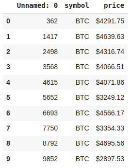
The code snippet below imports these libraries and fetches the dataset from the directory path given to the Pandas read_csv() method. The Pandas head() method prints relevant columns from the crypto data. The column "Unnamed: 0" represents the index value of each data point.

Output

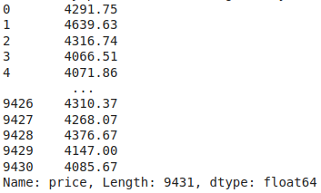
Next, we’ll clean the price column by removing the $ sign and converting the column type from string to float.

‍Output

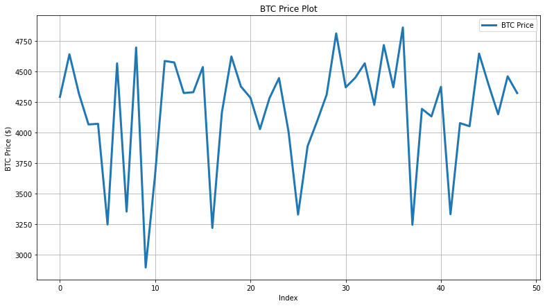
Now, let’s visualize the first 50 rows of the BTC price data, as we cannot fit the complete data in the plot. We can observe that the price of Bitcoin fluctuates between 3000 to 5000 in these records.

Output

Now, to use the BTC price data for calculating the moving averages, we’ll convert the Pandas "price" column to a NumPy array (btc_price) using the to_numpy() method, as shown in the code snippet below.

‍Output

‍

Our basic setup is complete. To experiment, we’ll calculate the 5-day and 20-day windows for SMA and EMA. CMA will be calculated on the entire dataset. Now, let’s calculate moving averages, starting with SMA. 

Calculating simple moving average using Python’s NumPy

In NumPy, SMA can be calculated using different coding approaches. We’ll look at three approaches below:

1. Using the numpy.sum() method
2. Using the numpy.convolve() method
3. Using the numpy.lib.stride_tricks.sliding_window_view() & numpy.average() methods

1. Using the numpy.sum() method

First, we’ll set the base window size to 5. We’ll define an SMA() method which sums all the values (v) within the current data window (n) using the np.sum() method and divides it by the current data window to obtain the simple moving average. The window continues to slide on the entire dataset using a while loop.

‍Output Plot

2. Using the numpy.convolve() method

The code snippet below defines a SMA_convolve() method, which uses the np.convolve() method to apply convolution. Convolution is a mathematical operation applied on two arrays or matrices to obtain a resultant array that captures the effect of one array over the other. 

Here it is applied to the values in the current window (n) with an array of 1’s. The resulting arrays contain simple moving averages for 5-day and 20-day windows. The output of this method is identical to the first method.

3. Using the numpy. lib.stride_tricks. sliding_window_view() & numpy.average ( ) methods

The code snippet below defines a SMA_sliding_window() method which uses the sliding_window_view() method from a NumPy module named stride_tricks. It automatically slides the window over the entire data array and averages the elements in each window using the np.average() method. The resulting arrays contain simple moving averages for 5-day and 20-day windows. The output of this method is identical to the first method.

Calculating cumulative moving average using numpy.cumsum() method

The code snippet below evaluates the cumulative moving average. We’ll start by defining the CMA() method. Then we’ll calculate the cumulative sum of the entire data array (btc_price). Next, we’ll iterate (i) through all the elements in the cumulative sum array until the current iteration. As iterations increase, the average calculations continue to add the next elements.

As the iterations increase, the value of CMA becomes more desensitized to any change in the data points. Think of it as the CGPA of a student. If the student performs well in the early semesters, the CGPA reflects the student’s performance appropriately. If the performance drops in the later semesters, the CGPA won’t show major deviations. Hence the impact of later semesters would be lesser in CGPA calculation. 

Now reverse it. A bad performance in early semesters greatly decreases the CGPA, but a good performance in later semesters doesn't have much impact. That’s how the cumulative moving average generally works.

‍Output Plot

Calculating exponential moving average using NumPy

Finally, we’ll calculate the exponential moving average by defining an  EMA() method that calculates the smoothing factor (alpha) value and uses it to give more weightage to the most recent elements in the data.

Here, for a 5-day EMA, the  alpha value is 0.33. For a 20-day EMA, the alpha value is 0.095. There are different methods for calculating this value. We have leveraged the commonly used sf = 2 / (n+1).

Output Plot

Visualizing & Comparing Different Moving Averages

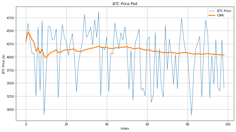
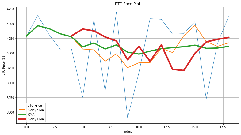
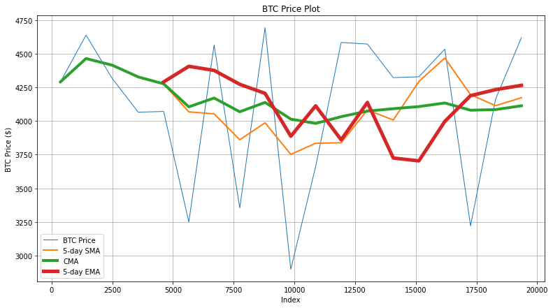
To observe how different MAs stack up against each other, we’ll plot comparison graphs using the Matplotlib library. The code snippet below generates a graph that shows the actual BTC price, 5-day SMA/EMA, and CMA values for the first 20 records.

Output

You can observe that the CMA curve is smoother than the rest because it averages the entire dataset progressively. However, since the BTC prices fluctuate more frequently in this dataset, CMA has lesser accuracy than SMA and EMA.

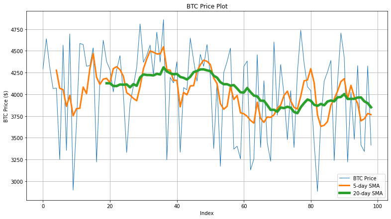
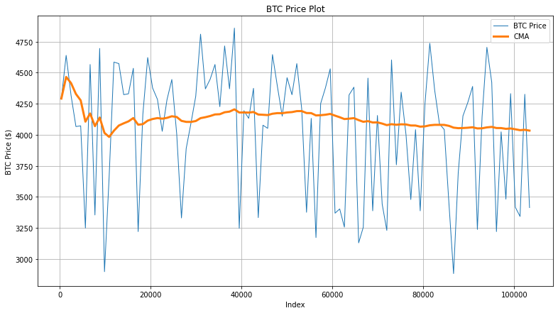
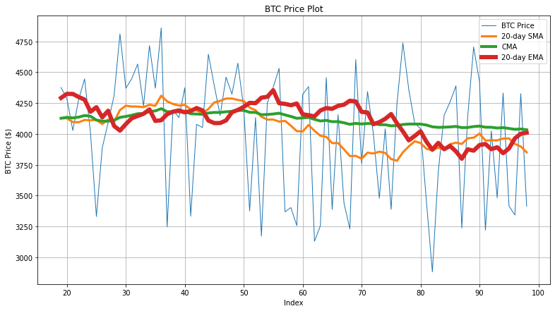
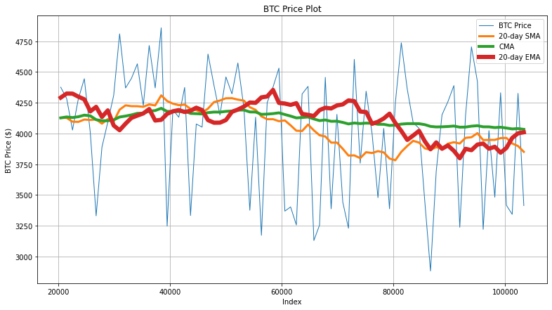
The next code snippet generates the graph that shows the actual BTC price, 20-day SMA/EMA, and CMA values for the first 100 records.

Output

Here, the 20-day EMA tries to capture the fluctuation of BTC more aggressively. However, since the fluctuations are frequent, the accuracy of EMA is not up to the mark.

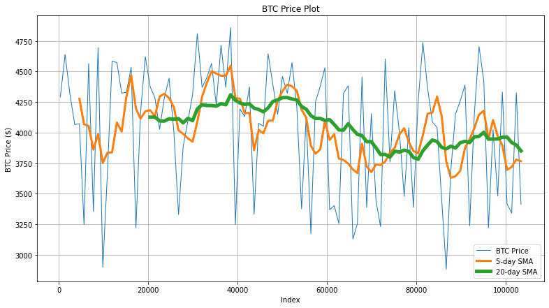
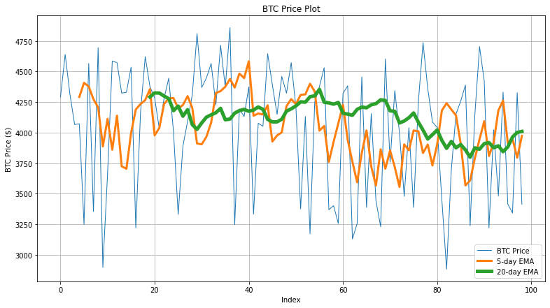
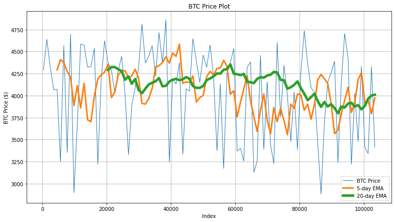
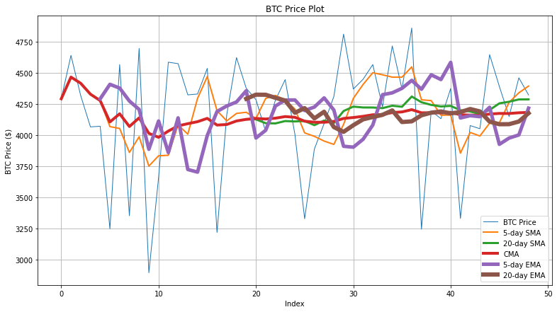
Finally, the code snippet below generates the graph that shows the actual BTC price, 5-day SMA/EMA, 20-day SMA/EMA, and CMA values for the first 50 records.

Output

Here, you can see the complete picture. Again, we can observe that 5-day and 20-day EMA tries to capture the BTC price fluctuations to some extent. But the actual price trends are very abrupt, which affects the accuracy of moving averages.

These experiments tell us that real-world data has a lot of complexities. Especially markets like crypto offer aggressive fluctuations, making it difficult to map this data using moving averages. This is one of the many limitations of MAs, which we’ll discuss next.

Simple moving average is less suitable for applications that rely on recent data for effective operations as SMA gives equal weightage to all elements in the sliding window. In these cases, EMA is better as it penalizes old or stale data and reacts faster to value changes. 

If the data shows cyclical behavior, such as moving up and down frequently, then the moving average may not be able to capture meaningful trends. If the data isn’t trending in either direction, MA cannot capture any valuable information.

Moreover, the variations in the size of the sliding window change the moving average measurement. If the dataset contains frequent fluctuations, a larger sliding window size would be more suitable for statistical analysis to smooth out the data.

However, there is no right or wrong sliding window size but the one that works for your statistical model. 

For instance, the most commonly used moving averages in stock trading are 10-day, 20-day, 50-day, 100-day, and 200-day. Some models may capture valuable trends in a 20-day window, while other long-term trends may only be noticeable in a 100-day moving average. For example, a stock trading above its 200-day SMA is considered in a long-term uptrend. This generates a BUY signal for analysts as the stock's overall health appears good.

Since the moving average is an average measurement, it does not record or show the data's extreme values (minimum and maximum). Hence, the statistical model loses its accuracy to some extent.

Additionally, moving averages must be combined with other statistical indicators in critical use cases such as stock trading. MA only accounts for historical trends in the stock price data. Some stock price analysts believe that past behavior is not an indicator of the future. So, combining technical stock indicators catering to momentum, volume, volatility, and breadth would analyze data robustly and make accurate stock price predictions.

Best practices for implementing moving average

You can get the most out of the moving average technique by following some essential best practices mentioned below.

Optimize sliding window size

Analysts can optimize the sliding window size to extract actionable trends to implement a moving average statistical model. They can compare the sliding window sizes' results to observe which preserves the most information. A better strategy is to dynamically adapt the sliding window size by periodically testing new data samples.

Account for outliers

Time series data often contain outliers. MA can filter out some of these outliers by reducing the obvious noise in the data. However, some outliers could be difficult to track due to abrupt changes in the data, such as a market that can become unstable quickly due to political activities, governmental policy changes, international monetary sanctions, or disruption in the supply and demand of products. In such cases, MA may not be the best choice for statistical analysis. Still, by carefully adjusting the moving window size, such outliers can be minimized to some extent.

Adjust weights as needed

By adjusting the weights of the MA, we can give more importance to specific data points and reduce the effect of data points that might be contributing adversely to MA calculations.

Conclusion

Moving average is one of the most common statistical indicators for analyzing trends in time-stamped data. MA reduces the noise in the data and presents a smooth-flowing line or curve that indicates the overall upward or downward trend in the data. As a result, the effect of outliers or noise on the data can be minimized. 

Data analysts can use Python’s NumPy library to calculate moving averages for time series or ordered data sequences. It offers different techniques to calculate SMA, CMA, and EMA. Analysts can adjust the sliding window size after carefully observing the trends captured by each window.